IV. Writing the data

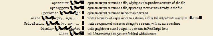
Files and pipes are both examples of general Mathematica objects known as streams. A stream in Mathematica is a source of input or output.

The basic low-level scheme for writing output to a stream in Mathematica is as follows. First, you call OpenWrite or OpenAppend to “open the stream”, telling Mathematica that you want to write output to a particular file or external program, and in what form the output should be written. Having opened a stream, you can then call Write or WriteString to write a sequence of expressions or strings to the stream. When you have finished, you call Close to “close the stream”.

Examples:

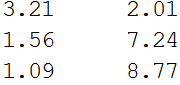
Let’s enter the data in two columns of numbers:

data1={{3.21, 2.01},{1.56, 7.24},{1.09, 8.77}}// TableForm

Then we’ll write the given data to a hard drive:

data2=OutputForm[data1];

stmp = OpenWrite["data1.txt"];

Write[stmp,data2]; Close[stmp];

As a result we can see the text file with data in corresponding Mathematica folder.

One can read it by using the ReadList operator:

data3=ReadList["data1.txt"]

{6.4521,11.2944,9.5593}

What has happened is that ReadList has interpreted each line of the file as a multiplication of two numbers, which Mathematica has evaluated. This can be suppressed by telling ReadList to read numbers.

data4=ReadList["data1.txt", Number]

{3.21,2.01,1.56,7.24,1.09,8.77}

If the numbers in the file represent { x, y } pairs, we can have ReadList handle each line separately by setting RecordLists to True.

data4=ReadList["data1.txt", Number, RecordLists->True]//TableForm

Or you can directly use the Import operator:

data5=Import["data1.txt"]

3.21 2.01

1.56 7.24

1.09 8.77

So, we received the initial data, written on the disk.

V. Entering the experimental data in Mathematica

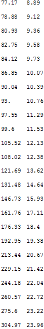
If we have lists of x and y values, given separately, we can enter them in such form:

X={77.17,78.88,80.93,82.75,84.12,86.85,90.04,93.,97.55, 99.6,105.52,108.02,121.69,131.48,146.73,161.76,176.33,192.95,

213.44,229.15,244.18,260.57,275.6,304.97};

Y={8.89,9.12,9.36,9.58,9.73,10.07,10.39,10.76,11.29,11.53,

12.13,12.38,13.62,14.64,15.93,17.11,18.4,19.38,20.67,21.42,22.0,22.72,23.22,23.96};

The next step is to combine them in one array:

data1=Table[{X,Y}]

dat2=TableForm[%, TableDirections->{Row,Column}]

This gives:

{{77.17,78.88,80.93,82.75,84.12,86.85,90.04,93.,97.55,99.6,105.52,108.02,121.69,131.48,146.73,161.76,176.33,192.95,213.44,229.15,244.18,260.57,275.6,304.97},{8.89,9.12,9.36,9.58,9.73,10.07,10.39,10.76,11.29,11.53,12.13,12.38,13.62,14.64,15.93,17.11,18.4,19.38,20.67,21.42,22.04,22.72,23.22,23.96}}

So, we constructed the necessary data array, that can be used in ListPlot, Fit and other Mathematica operators.

Homework 1/9

Enter the correspondent lists of x and y values separately, construct the data array with two columns, write it as the *.txt file, then read to the Math-file, plot by ListPlot operator and write figure as the *jpg file at the hard drive.

VI. Getting Data from a Scanned Plot (Appendix 1)

Sometimes we wish to analyze data taken by somebody else, such as might be found in a journal or book. However, many times only a graph of the data is printed. If the highest precision is required, then one must usually write to the original source and request the actual numbers. Often, however, approximate numbers that are directly available from the plot are close enough.

Provided you have access to a scanner, the Mathematica front end provides capabilities to extract those numbers, and this section is a tutorial in using that capability. The format of the scan file that can be recognized by the front end is dependent on the computer on which it is running; consult the documentation for your front end for further information. In addition, we will be using the front end's ability to select points in a graphic and to cut-and-paste the coordinates into an input cell; again, the exact details of how to do this will depend on the computer being used.

We will use as an example a plot whose result is known: a plot generated by ListPlot that appears on page 487 of Stephen Wolfram's The Mathematica Book, 4th edition (Wolfram Media and Cambridge Univ. Press, 1999). After scanning the relevant page from the book, we will import it into the notebook.

We will first locate the graphics coordinates of the x axis at zero and 20. The actual numbers were generated by cutting and pasting from the graphic; everything else was typed in by hand.

In[1]:=

In[2]:=

The conversion from graphics coordinates to the actual units of the x axis is linear.

Now we evaluate the numbers.

In[3]:=

Out[3]=

In[4]:=

Out[4]=

We similarly convert graphics coordinates to the units of the y axis.

In[5]:=

Finally, we extract the coordinates of the data points.

Then the x values, converted to the units of the plot, can be calculated.

In[10]:=

Out[10]=

This compares well with the actual integers 1, 2,..., 19, 20.

We similarly find the y values.

In[11]:=

Out[11]=

These are within a few percent of the actual numbers.

In[12]:=

Out[12]=

We plot the scanned data results.

In[13]:=

In[14]:=

Дата добавления: 2014-01-11