Criterion of a consent of Kolmogorov

Probabilistic and statistical aspects of imitating modeling

Often mathematical models of the systems interesting us contain accidental parameters of their functioning and/or accidental external impacts.

Example 2.1. Work of a hairdressing salon is researched. Accidental external impacts – time intervals between the next visitors δ1, δ2, …. Accidental parameters of functioning – times τ1 (l), τ2 (l), … servicing of the next clients of l – m the hairdresser. A research purpose – to solve, how many to hire hairdressers that the average time of expectation in queue didn't exceed the set size. For this purpose it is necessary to lose some working days (are accelerated) and to look what will be queue in case of different number of hairdressers. To lose day of work, it will be required to generate specific values d1, d2, … sizes δ1, δ2, …. We will consider that δ1, δ2, … – the independent, equally distributed random variables: i.e. d1, d2, … – implementation of selection of distribution.

For some random variables, we will tell δ, we assume a certain type of distribution, for example exponential, for others (τ1 (l)) a type of distribution isn't clear, and there is a task of check of a hypothesis that this some fixed (standard) distribution which we assume.

The main ("zero") hypothesis consists that function of distribution of a random variable ξ is some fixed function

, (1)

alternative hypothesis – distribution function another:

. (2)

For check of these hypotheses we use selection of supervision of size ξ:

. (3)

Empirical function of distribution:

.

If H ₀ is fair, must be close to and backwards, that is size will be indicative – the maximum deviation of empirical function of distribution from the hypothetical.it is accidental, as selection on which is calculated , I could be different. Great values in advantage H ₁, therefore significance value of specific data , which led to the specific , against a hypothesis H ₀, equals

.

Kolmogorovs Theorem. If is continuous, that distribution of statistics , on condition of justice of Н ₀, doesn't depend from also is called as Kolmogorov's distribution with N degrees of freedom.

Example 2.2. On selection to check a hypothesis Н ₀: – uniform distribution on a piece [1, 5] (U (1, 5)).

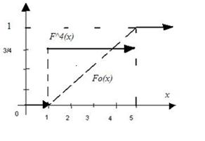
From picture

We can see, that d ₄ = ¾. .

According to tables [7, table 6.2] we find SL <0.01 (0.01 precisely for 0.734). Such significance value of data is interpreted as "the high importance, H0 almost for certain doesn't prove to be true", ξhas no distribution of U(1, 5).

Kolmogorovs Theorem.. .

K(x) is called Kolmogorovs distribution [7, table 6.1].

already in case of N > 20.

Example 2.2 (continuation):

As empirical function of distribution is step, and not decreasing, then it is the share of one of function gap points .

Consent criteria χ2

Hypotheses (1), (2) according to data (3) are again checked. Algorithm of actions:

We will break area of possible values of a random variable ξon H₀ on

r of intervals k = 1,…, r.

To these intervals on distribution of H₀ there correspond probabilities of hit ξ in them .

ν _k – number of supervision (sample units) which got to k-y an interval

(), (4)

– frequency of hits in an interval.

Compare statistics . In case of accomplishment of H₀ of frequency will be close to the corresponding probabilities therefore small values of statistics of H² therefore great values witness against H₀ are expected.

, – the observed (actually received) value of statistics of H².

Pearsons Theorem.

In case of justice of H0 distribution of statistics of H2 aims in case of to distribution χ² with r – 1 degrees of freedom.

Heuristic proof:

according to Moivre – Laplace theorem

,

, that is has distribution χ2 with r freedom degrees (actually r – 1 as on (4) νr depends on the others).

According to Pearsons theorem

. (5)

Owing to approximate nature of a formula (5) it is desirable to provide , , n_k – numbers of sample units in intervals (can be, for this purpose it is necessary to unite intervals).

Ifit isn't completely determined and l of its unknown parameters were estimated on initial selection, the number of degrees of freedom in (5) needs to be reduced to r – 1 – l.

Definition. Diagram like function from – average points of intervals, is called as the histogram.

We will check H₀ hypothesis that – normal distribution with the parameters estimated on the same selection (curve fo (y)).

p ₁ = F ₀(4) – F ₀(-∞) = 0.262, p ₂ = F ₀(5) – F ₀(4) = 0.252, p ₃ = 0.246, p ₄ = 0.156,

p ₅ = 0.084.

,

.

SL is great (> 0.1), data aren't significant against H₀, it could be supervision of a normal random variable.

Generation of the pseudorandom numbers which are regularly distributed on a piece [0, 1]

Carrying out imitation will require implementation

(6)

distributions . Distributions will be necessary different, for a start let it will be U(0, 1).

Practically we receive numbers (6) by consecutive appeals to some sensor which can be the physical device connected with a case or the computer program which develops various numbers. In the latter case these numbers call pseudorandom with distribution , if they meet conditions which are expected from selection of distribution . Pseudorandom (allegedly accidental) as truly accidental they aren't (can be always repeatedly received).

Thus, we expect (and it is necessary to check it) from pseudorandom numbers with distribution of U(0, 1):

– uniformity, i.e. consent with distribution of U(0, 1).

– accident.

Criterion of accident

Let there is an ordered set of numbers

(7)

(or a train – final sequence).

Definition. The train is called accidental if it is selection implementation.

According to data (7) it is necessary to check a hypothesis ,

that is the independent equally distributed random variables, in case of alternative of H₁ it not so.

We will consider in the beginning a case when elements in (7) can be only two types (1 and 0, And and In,…).

Example 2.7. Train 10100011010.

In really random check of this kind we don't expect that all "1" will get off together, and we don't expect that they will regularly alternate with "0".

In a train of elements of two types the set of the going in a row identical elements limited to opposite elements, either the beginning, or end is called as a series.

As statistics of criterion we will choose a random number of series K. We will designate: N₁ – number of elements than which in a train it is less; N₂ – number of elements than which in a train it is more.

It is possible to show that in case of justice of H₀ . Means, strong deviations of number of series from MK – for benefit of H₁ hypothesis.

SL (k) = P { K = k or further away from MK (all "tail") + K belongs to opposite "tail" with the same probability | H₀ }.

In case of the fixed SL = α it is possible to tabulate sizes и such that in case of the reached SL will be > α.

Example 2.7 (continuation): N₁ = 5, N₂ = 6, number of series k = 8.

According to the table of distribution of K [7, table 6.7]:

=> SL > 0.05;

=> SL > 0.1.

Means, SL> 0.1, data aren't significant against H₀, the train is accidental.

If either N₁, or N₂> 20, statistics

in case of H₀ has normal standard distribution is approximate. Therefore

. (8)

Now let numbers (7) – allegedly selection of arbitrary continuous distribution. It is possible to resolve an issue of not accident of this train as follows.

We will remember: a median – a quantile about 0.5; the selective median of M e is equal to a median element of a variational series if number of supervision odd, and it is equal to a floor the amount of 2 median elements of a variational series if number of supervision even. We will constitute differences , then instead of (7) we have a train of signs + and – which accident we are able to check.

If the train (7) accidental, consecutive excess of a median is independent events and the train of signs will be accidental therefore if a train of signs the nonrandom, and initial train wasn't accidental.

Multiplicative congruent method generation pseudorandom Numbers

Let x _{n -1} - a number (0, 1). Obtain , Where β - large integer; D - taking the fractional part (discard the integer part, if there is one). The new number x _n Again from (0.1) it again multiplied by β and t. d., get the sequence of numbers uniformly distributed nnyh g on (0, 1).

The algorithm can be rewritten. Let a _n - integer, M - large integer,

, (9)

. (10)

Definition. Alance of the division of a natural number p by a positive integer q denotes (p) mod q.

Formula (10) can be rewritten

, n = 1, 2, …. (11)

algorithm is (11), (9) easier to implement on a computer.

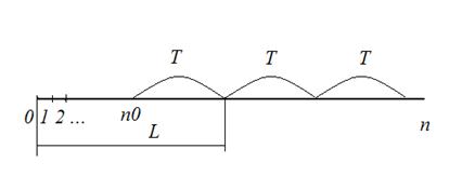
The sequence P (11) always loops, ie. e. beginning with some n = ₀ to the period length T, which then repeats endlessly smiling. L - length of the segment aperiodicity.

Дата добавления: 2014-10-23