Calculating the p-value, ctd

· To compute the p -value, you need the to know the sampling distribution of , which is complicated if n is small.

· If n is large, you can use the normal approximation (CLT):

p -value = ,

=

=

@ probability under left+right N (0,1) tails

where = std. dev. of the distribution of = s_Y /.

Calculating the p-value with s_Y known:

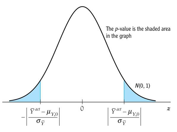
· For large n, p -value = the probability that a N (0,1) random variable falls outside |(– m_{Y ,0})/|

· In practice, is unknown – it must be estimated

Estimator of the variance of Y:

= = “sample variance of Y ”

Fact:

If (Y ₁,…, Y_n) are i.i.d. and E (Y ⁴) < ¥, then

Why does the law of large numbers apply?

· Because is a sample average; see Appendix 3.3

· Technical note: we assume E (Y ⁴) < ¥ because here the average is not of Y_i, but of its square; see App. 3.3

Computing the p-value with estimated:

p -value = ,

=

@ (large n)

so

p -value = ( estimated)

@ probability under normal tails outside | t^act |

where t = (the usual t -statistic)

What is the link between the p -value and the significance level?

The significance level is prespecified. For example, if the prespecified significance level is 5%,

· you reject the null hypothesis if | t | ³ 1.96

· equivalently, you reject if p £ 0.05.

· The p -value is sometimes called the marginal significance level.

· Often, it is better to communicate the p -value than simply whether a test rejects or not – the p -value contains more information than the “yes/no” statement about whether the test rejects.

At this point, you might be wondering,...

What happened to the t -table and the degrees of freedom?

Digression: the Student t distribution

If Y_i, i = 1,…, n is i.i.d. N (m_Y,), then the t -statistic has the Student t -distribution with n – 1 degrees of freedom.

The critical values of the Student t -distribution is tabulated in the back of all statistics books. Remember the recipe?

1. Compute the t -statistic

2. Compute the degrees of freedom, which is n – 1

3. Look up the 5% critical value

4. If the t -statistic exceeds (in absolute value) this critical value, reject the null hypothesis.

Comments on this recipe and the Student t -distribution

1. The theory of the t -distribution was one of the early triumphs of mathematical statistics. It is astounding, really: if Y is i.i.d. normal, then you can know the exact, finite-sample distribution of the t -statistic – it is the Student t. So, you can construct confidence intervals (using the Student t critical value) that have exactly the right coverage rate, no matter what the sample size. This result was really useful in times when “computer” was a job title, data collection was expensive, and the number of observations was perhaps a dozen. It is also a conceptually beautiful result, and the math is beautiful too – which is probably why stats profs love to teach the t -distribution. But….

Comments on Student t distribution, ctd.

2. If the sample size is moderate (several dozen) or large (hundreds or more), the difference between the t -distribution and N(0,1) critical values are negligible. Here are some 5% critical values for 2-sided tests:

degrees of freedom (n – 1)	5% t -distribution critical value
	2.23
	2.09
	2.04
	2.00
¥	1.96

Comments on Student t distribution, ctd.

3. So, the Student- t distribution is only relevant when the sample size is very small; but in that case, for it to be correct, you must be sure that the population distribution of Y is normal. In economic data, the normality assumption is rarely credible. Here are the distributions of some economic data.

· Do you think earnings are normally distributed?

· Suppose you have a sample of n = 10 observations from one of these distributions – would you feel comfortable using the Student t distribution?

Comments on Student t distribution, ctd.

4. You might not know this. Consider the t -statistic testing the hypothesis that two means (groups s, l) are equal:

Even if the population distribution of Y in the two groups is normal, this statistic doesn’t have a Student t distribution!

There is a statistic testing this hypothesis that has a normal distribution, the “pooled variance” t -statistic – see SW (Section 3.6) – however the pooled variance t -statistic is only valid if the variances of the normal distributions are the same in the two groups. Would you expect this to be true, say, for men’s v. women’s wages?

The Student-t distribution – summary

· The assumption that Y is distributed N (m_Y,) is rarely plausible in practice (income? number of children?)

· For n > 30, the t -distribution and N (0,1) are very close (as n grows large, the t_{n –1} distribution converges to N (0,1))

· The t -distribution is an artifact from days when sample sizes were small and “computers” were people

· For historical reasons, statistical software typically uses the t -distribution to compute p -values – but this is irrelevant when the sample size is moderate or large.

· For these reasons, in this class we will focus on the large- n approximation given by the CLT

1. The probability framework for statistical inference

2. Estimation

3. Testing

Дата добавления: 2014-01-07