КАТЕГОРИИ:
Архитектура-(3434)Астрономия-(809)Биология-(7483)Биотехнологии-(1457)Военное дело-(14632)Высокие технологии-(1363)География-(913)Геология-(1438)Государство-(451)Демография-(1065)Дом-(47672)Журналистика и СМИ-(912)Изобретательство-(14524)Иностранные языки-(4268)Информатика-(17799)Искусство-(1338)История-(13644)Компьютеры-(11121)Косметика-(55)Кулинария-(373)Культура-(8427)Лингвистика-(374)Литература-(1642)Маркетинг-(23702)Математика-(16968)Машиностроение-(1700)Медицина-(12668)Менеджмент-(24684)Механика-(15423)Науковедение-(506)Образование-(11852)Охрана труда-(3308)Педагогика-(5571)Полиграфия-(1312)Политика-(7869)Право-(5454)Приборостроение-(1369)Программирование-(2801)Производство-(97182)Промышленность-(8706)Психология-(18388)Религия-(3217)Связь-(10668)Сельское хозяйство-(299)Социология-(6455)Спорт-(42831)Строительство-(4793)Торговля-(5050)Транспорт-(2929)Туризм-(1568)Физика-(3942)Философия-(17015)Финансы-(26596)Химия-(22929)Экология-(12095)Экономика-(9961)Электроника-(8441)Электротехника-(4623)Энергетика-(12629)Юриспруденция-(1492)Ядерная техника-(1748)
Monopoly Profit Maximization
|
|
|
|
The profit received by the firm equals the total revenue minus the total cost. In the figure, we can see that if quantity q1 is produced, the total revenue is TR1 and total cost is TC1. The difference, TR1 – TC1, is the profit received. The same is depicted by the length of the line segment AB, i.e., the vertical distance between the TR and TC curves at q1 level of output. It should be clear that this vertical distance changes for diferent levels of output.
When output level is less than q2, the TC curve lies above the TR curve, i.e., TC is greater than TR, and therefore profit is negative and the firm makes losses.
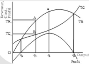
The same situation exists for output levels greater than q3. Hence, the firm can make positive profits only at output levels between q2 and q3, where TR curve lies above the TC curve. The monopoly firm will choose that level of output which maximises its profit. This would be the levelof output for which the vertical distance between the TR and TC is maximum and TR is above the TC, i.e., TR – TC is maximum. This occurs at the level of output q0. If the difference TR – TC is calculated and drawn as a graph, it will look as in the curve marked ‘Profit’ in Figure 3. It should be noticed that the Profit curve has its maximum value at the level of output q0.
The analysis shown above can also be conducted using Average and Marginal Revenue and Average and Marginal Cost. Though a bit more complex, this method is able to exhibit the process in greater light.
In Figure 4, the Average Cost (AC), Average Variable Cost (AVC) and Marginal Cost (MC) curves are drawn along with the Demand (Average Revenue) Curve and Marginal Revenue curve.
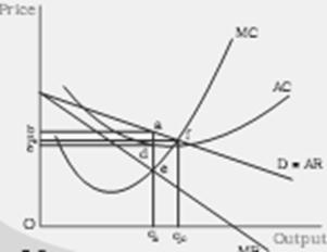
The rule for monopoly profit maximization will come as no surprise. It is
MR=MC
That is, the rule says that the monopoly should increase output up to the level where the marginal cost curve intersects the marginal revenue curve, in order to maximize its profits. The price charged is the corresponding price on the demand curve. Notice that this is a two-stage analysis:
– at the first stage, the marginal cost, shown in red, and the marginal revenue, shown in light green determine the output. Profit maximizing output is the output at which they intersect, shown by the gold line.
– at the second stage, the output and the demand curve determine the price. Trace up the vertical gold line to the dark green demand curve, and that's the profit-maximizing price. The diagram is a little more complex. Here it is:
|
|
|
|
|
Дата добавления: 2014-01-11; Просмотров: 742; Нарушение авторских прав?; Мы поможем в написании вашей работы!