К Лекции 8

Иллюстрации к технике Паунда-Дривера-Холла

Am. J. Phys., Vol. 69, No. 1, January 2001 Eric D. Black

Fig. 1. Transmission of a Fabry–Perot cavity vs frequency of the incident

light. This cavity has a fairly low finesse, about 12, to make the structure of

the transmission lines easy to see.

Fig. 2. The reflected light intensity from a Fabry–Perot cavity as a function

of laser frequency, near resonance. If you modulate the laser frequency, you

can tell which side of resonance you are on by how the reflected power

changes.

Fig. 3. The basic layout for locking a cavity to a laser. Solid lines are optical

paths and dashed lines are signal paths. The signal going to the laser controls

its frequency.

Fig. 4. Magnitude and phase of the reflection coefficient for a Fabry–Perot

cavity. As in Fig. 1, the finesse is about 12. Note the discontinuity in phase,

caused by the reflected power vanishing at resonance.

Fig. 6. The Pound–Drever–Hall error signal, e /2A PcPs vs v/Dn fsr, when

the modulation frequency is low. The modulation frequency is about half a

linewidth: about 1023 of a free spectral range, with a cavity finesse of 500.

Fig. 7. The Pound–Drever–Hall error signal, e /2A PcPs vs v/Dn fsr, when

the modulation frequency is high. Here, the modulation frequency is about

20 linewidths: roughly 4% of a free spectral range, with a cavity finesse of

500.

Иллюстрации к технике Оптической Гребенки и применению в астрономических спектрографах высокого разрешения

Figure 1: Sketch of the experimental setup at the VTT. By superimposing the frequency comb with light from a celestial body – in this case, the Sun – one can effectively calibrate its emission or absorption spectrum against an atomic clock. An erbium-doped fiber LFC with 250-MHz mode spacing (pulse repetition rate) is filtered with a FPC to increase the effective mode spacing, allowing it to be resolved by the spectrograph. The latter has a resolution of _0.8 GHz at wavelengths around 1.5 μm, where our LFC tests were conducted. The LFC was controlled by a rubidium atomic clock. A continuous-wave (CW) laser at 1583 nm was locked to one comb line and simultaneously fed to a wavemeter. Even though the wavemeter is orders of magnitude less precise than the LFC itself, it is sufficiently accurate (better than 250 MHz) to identify the mode number, n. The FPC length, defining the final free spectral range (FSR), was controlled by feedback from its output. See (10) for further details.

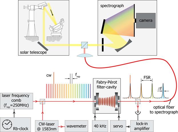
Figure 1: Sketch of our experimental setup at the VTT. By superimposing the frequency comb

with light from a celestial body – in this case, the Sun – one can effectively calibrate its emission

or absorption spectrum against an atomic clock. An erbium-doped fiber LFC with 250-MHz

mode spacing (pulse repetition rate) is filtered with a FPC to increase the effective mode spacing, allowing it to be resolved by the spectrograph. The latter has a resolution of _0.8 GHz at

wavelengths around 1.5 μm, where our LFC tests were conducted. The LFC was controlled by

a rubidium atomic clock. A continuous-wave (CW) laser at 1583 nm was locked to one comb

line and simultaneously fed to a wavemeter. Even though the wavemeter is orders of magnitude

less precise than the LFC itself, it is sufficiently accurate (better than 250 MHz) to identify the

mode number, n. The FPC length, defining the final free spectral range (FSR), was controlled

by feedback from its output. See (10) for further details.

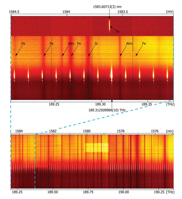
Figure 2: Spectra of the solar photosphere (background image) overlaid by a LFC with 15 GHz

mode spacing (white, equally spaced vertical stripes). Spectra are dispersed horizontally,

whereas the vertical axis is a spatial cross section of the Sun’s photosphere. The upper panel

shows a small section of the larger portion of the spectrum below. The brighter mode labeled

with its absolute frequency is additionally superimposed with a CW laser used to identify the

mode number (Fig. 1). The frequencies of the other modes are integer multiples of 15 GHz

higher (right) and lower (left) in frequency. Previous calibration methods would use the atmospheric absorption lines (dark vertical bands labeled “Atm” interleaved with the Fraunhofer

absorption lines), which are comparably few and far between. Also shown in the upper panel

is the only thorium emission line lying in this wavelength range from a typical hollow-cathode

calibration lamp. Recording it required an integration time of 30 min, compared with the LFC

exposure time of just 10 ms. Unlike with the LFC, the thorium calibration method cannot be

conducted simultaneously with solar measurements at the VTT. The nominal horizontal scale

is 1.5×10−3 nm pixel−1 with _1000 pixels shown horizontally in the upper panel. Black horizontal

and vertical lines are artifacts of the detector array

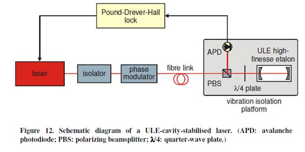
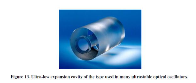
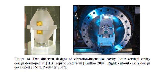
Иллюстрации к технике оптических эталонов частоты

Дата добавления: 2014-01-11