Chapter 04.06

GaussianElimination

After reading this chapter, you should be able to:

1. Solve a set of simultaneous linear equations using Naïve Gauss Elimination,

1. Learn the pitfalls of Naïve Gauss Elimination Method,
2. Understand the effect of round off error on a solving set of linear equation by Naïve Gauss Elimination Method,
3. Learn how to modify Naïve Gauss Elimination method to Gaussian Elimination with Partial Pivoting Method to avoid pitfalls of the former method,
4. Find the determinant of a square matrix using Gaussian Elimination,
5. Understand the relationship between determinant of co-efficient matrix and the solution of simultaneous linear equations.

How are a set of equations solved numerically?

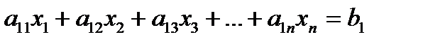
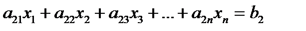
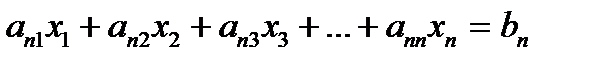
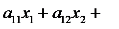
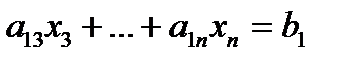
One of the most popular techniques for solving simultaneous linear equations is the Gaussianelimination method. The approach is designed to solve a general set of n equations and n unknowns

..

..

..

Gaussianelimination consists of two steps

1. Forward Elimination of Unknowns: In this step, the unknown is eliminated in each equation starting with the first equation. This way, the equations are “reduced” to one equation and one unknown in each equation.

2. Back Substitution: In this step, starting from the last equation, each of the unknowns is found.

Forward Elimination of Unknowns:

In the first step of forward elimination, the first unknown, x₁ is eliminated from all rows below the first row. The first equation is selected as the pivot equation to eliminate x_{1 .} So, to eliminate x₁ in the second equation, one divides the first equation by a₁₁ (hence called the pivot element) and then multiply it by a₂₁. That is, same as multiplying the first equation by a₂₁ / a₁₁ to give

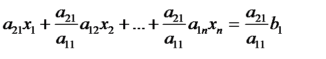
Now, this equation can be subtracted from the second equation to give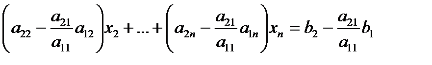

or

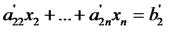
where

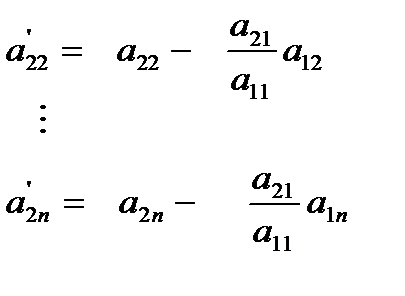
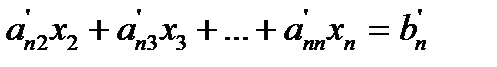
This procedure of eliminating , is now repeated for the third equation to the n^th equation to reduce the set of equations as

...

...

...

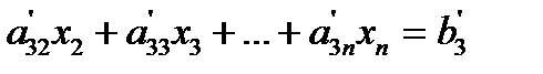
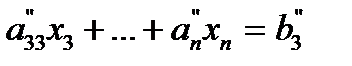
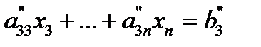
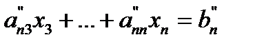
This is the end of the first step of forward elimination. Now for the second step of forward elimination, we start with the second equation as the pivot equation and as the pivot element. So, to eliminate x₂ in the third equation, one divides the second equation by (the pivot element) and then multiply it by . That is, same as multiplying the second equation by 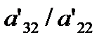and subtracting from the third equation. This makes the coefficient of x₂ zero in the third equation. The same procedure is now repeated for the fourth equation till the nth equation to give

..

..

..

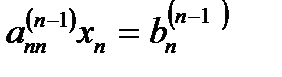
The next steps of forward elimination are conducted by using the third equation as a pivot equation and so on. That is, there will be a total of (n -1) steps of forward elimination. At the end of (n -1) steps of forward elimination, we get a set of equations that look like

..

..

..

Back Substitution:

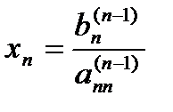
Now the equations are solved starting from the last equation as it has only one unknown.

Then the second last equation, that is the (n -1) ^th equation, has two unknowns - x_n and x_{n -1}, but x_n is already known. This reduces the (n -1) ^th equation also to one unknown. Back substitution hence can be represented for all equations by the formula

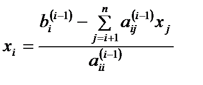for i = n – 1, n – 2,…,

and

Дата добавления: 2014-12-27