Estimation

Randomness and data

We will assume simple random sampling

Conditional mean, ctd.

Conditional expectations and conditional moments

Conditional distributions

· The distribution of Y, given value(s) of some other random variable, X

· Ex: the distribution of test scores, given that STR < 20

· conditional mean = mean of conditional distribution

= E (Y | X = x) (important concept and notation)

· conditional variance = variance of conditional distribution

· Example: E (Test scores | STR < 20) = the mean of test scores among districts with small class sizes

The difference in means is the difference between the means of two conditional distributions:

D = E (Test scores | STR < 20) – E (Test scores | STR ≥ 20)

Other examples of conditional means:

· Wages of all female workers (Y = wages, X = gender)

· Mortality rate of those given an experimental treatment (Y = live/die; X = treated/not treated)

· If E (X | Z) = const, then corr(X, Z) = 0 (not necessarily vice versa however)

The conditional mean is a (possibly new) term for the familiar idea of the group mean
(d) Distribution of a sample of data drawn randomly

from a population: Y B _{1 B} ,…, Y B _{n B}

· Choose and individual (district, entity) at random from the population

· Prior to sample selection, the value of Y is random because the individual selected is random

· Once the individual is selected and the value of Y is observed, then Y is just a number – not random

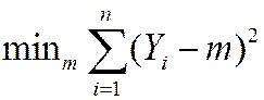
· The data set is (Y B_1B, Y B_2B,…, Y B _{n B}), where Y B _{i B} = value of Y for the i P^thP individual (district, entity) sampled

Distribution of Y B _{1 B} ,…, Y B _{n B} under simple random sampling

· Because individuals #1 and #2 are selected at random, the value of Y B_1B has no information content for Y B_2B. Thus:

o Y B_1B and Y B_2B are independently distributed

o Y B_1B and Y B_2B come from the same distribution, that is, Y B_1B, Y B_2B are identically distributed

o That is, under simple random sampling, Y B_1B and Y B_2B are independently and identically distributed (i.i.d.).

o More generally, under simple random sampling, { Y B _{i B}}, i = 1,…, n, are i.i.d.

This framework allows rigorous statistical inferences about moments of population distributions using a sample of data from that population …

1. The probability framework for statistical inference

3. Testing

4. Confidence Intervals

Estimation

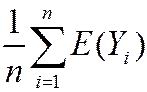
is the natural estimator of the mean. But:

(a) What are the properties of ?

(b) Why should we use rather than some other estimator?

· Y B_1B (the first observation)

· maybe unequal weights – not simple average

· median(Y B_1B,…, Y B _{n B})

The starting point is the sampling distribution of …

(a) The sampling distribution of

is a random variable, and its properties are determined by the sampling distribution of

· The individuals in the sample are drawn at random.

· Thus the values of (Y B_1B,…, Y B _{n B}) are random

· Thus functions of (Y B_1B,…, Y B _{n B}), such as , are random: had a different sample been drawn, they would have taken on a different value

· The distribution of over different possible samples of size n is called the sampling distribution of .

· The mean and variance of are the mean and variance of its sampling distribution, E () and var().

· The concept of the sampling distribution underpins all of econometrics.

The sampling distribution of , ctd.

Example: Suppose Y takes on 0 or 1 (a Bernoulli random variable) with the probability distribution,

Pr[ Y = 0] =.22, Pr(Y =1) =.78

Then

E (Y) = p ´1 + (1 – p)´0 = p =.78

= E [ Y – E (Y)]² = p (1 – p) [remember this?]

=.78´(1–.78) = 0.1716

The sampling distribution of depends on n.

Consider n = 2. The sampling distribution of is,

Pr( = 0) =.22² =.0484

Pr( = ½) = 2´.22´.78 =.3432

Pr( = 1) =.78² =.6084

The sampling distribution of when Y is Bernoulli (p =.78):

Things we want to know about the sampling distribution:

· What is the mean of ?

o If E () = true m =.78, then is an unbiased estimator of m

· What is the variance of ?

o How does var() depend on n (famous 1/ n formula)

· Does become close to m when n is large?

o Law of large numbers: is a consistent estimator of m

· – m appears bell shaped for n large…is this generally true?

o In fact, – m is approximately normally distributed for n large (Central Limit Theorem)

The mean and variance of the sampling distribution of

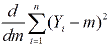
General case – that is, for Y_i i.i.d. from any distribution, not just Bernoulli:

mean: E () = E () = = = m_Y

Variance: var() = E [– E ()]²

= E [– m_Y ]²

= E

= E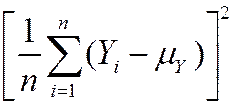

so var() = E

=

=

=

=

=

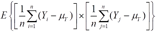
Mean and variance of sampling distribution of , ctd.

E () = m_Y

var() =

Implications:

1. is an unbiased estimator of m_Y (that is, E () = m_Y)

2. var() is inversely proportional to n

· the spread of the sampling distribution is proportional to 1/

· Thus the sampling uncertainty associated with is proportional to 1/(larger samples, less uncertainty, but square-root law)

The sampling distribution of when n is large

For small sample sizes, the distribution of is complicated, but if n is large, the sampling distribution is simple!

1. As n increases, the distribution of becomes more tightly centered around m_Y (the Law of Large Numbers)

2. Moreover, the distribution of – m_Y becomes normal (the Central Limit Theorem)

The Law of Large Numbers:

An estimator is consistent if the probability that its falls within an interval of the true population value tends to one as the sample size increases.

If (Y ₁,…, Y_n) are i.i.d. and < ¥, then is a consistent estimator of m_Y, that is,

Pr[| – m_Y | < e ] ® 1 as n ® ¥

which can be written, m_Y

(“ m_Y ” means “ converges in probability to m_Y ”).

(the math: as n ® ¥, var() = ® 0, which implies that Pr[| – m_Y | < e ] ® 1.)

The Central Limit Theorem (CLT):

If (Y ₁,…, Y_n) are i.i.d. and 0 < < ¥, then when n is large the distribution of is well approximated by a normal distribution.

· is approximately distributed N (m_Y, ) (“normal distribution with mean m_Y and variance / n ”)

· (– m_Y)/ s_Y is approximately distributed N (0,1) (standard normal)

· That is, “standardized” = = is approximately distributed as N (0,1)

· The larger is n, the better is the approximation.

Sampling distribution of when Y is Bernoulli, p = 0.78:

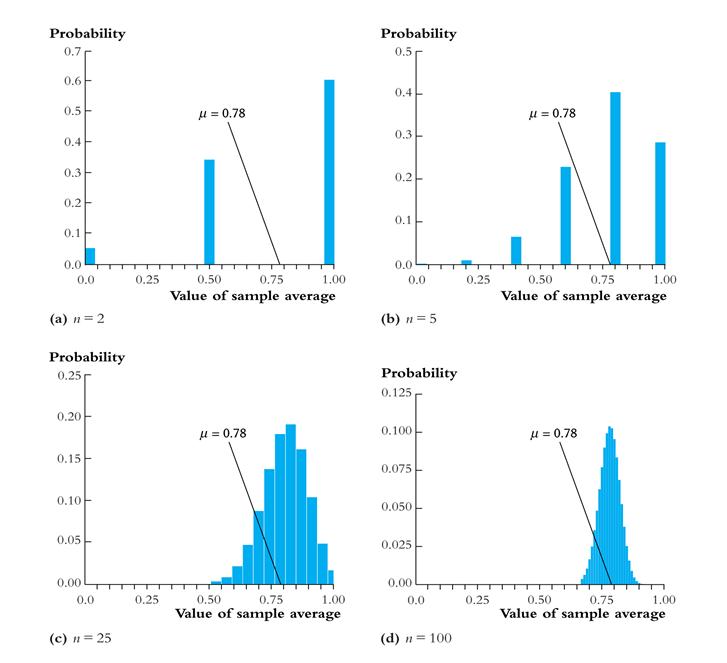
Same example: sampling distribution of :

Summary: The Sampling Distribution of

For Y ₁,…, Y_n i.i.d. with 0 < < ¥,

· The exact (finite sample) sampling distribution of has mean m_Y (“is an unbiased estimator of m_Y ”) and variance / n

· Other than its mean and variance, the exact distribution of is complicated and depends on the distribution of Y (the population distribution)

· When n is large, the sampling distribution simplifies:

o m_Y (Law of large numbers)

o is approximately N (0,1) (CLT)

(b) Why Use To Estimate m_Y?

· isunbiased: E () = m_Y

· is consistent: m_Y

· is the “least squares” estimator of m_Y; solves,

so, minimizes the sum of squared “residuals”

optional derivation (also see App. 3.2)

= =

Set derivative to zero and denote optimal value of m by :

= = or = =

Why Use To Estimate m_Y, ctd.

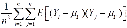
· has a smaller variance than all other linear unbiased estimators: consider the estimator, , where { a_i } are such that is unbiased; then var() £ var() (proof: SW, Ch. 17)

· isn’t the only estimator of m_Y – can you think of a time you might want to use the median instead?

1. The probability framework for statistical inference

2. Estimation

Дата добавления: 2014-01-07